Geochemical Clustering

This demo walks through a complete geochemical clustering workflow applied to whole-rock geochemical data. The goal is to identify distinct geochemical groups from multi-element assay data using a combination of compositional data transformation, dimensionality reduction, and unsupervised clustering.

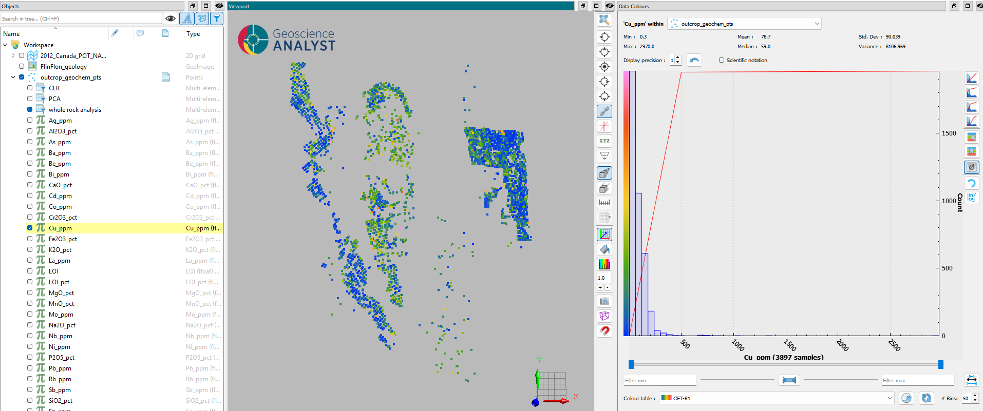
Fig. 15 Spatial distribution of whole-rock geochemical sample locations used in this demo.

The dataset consists of whole-rock major and trace element concentrations measured at sample locations around then well-known copper-zinc VMS deposit the Flin Flon mine in northern Manitoba, Canada. A total of 33 major and trace elements are included in the analysis, with concentrations reported in a mix of weight percent (wt%) for major oxides and parts per million (ppm) for trace elements. The samples are spatially distributed across the deposit area, providing a representative coverage of the geochemical variability.

Note

[Downloaded here] the geoh5 project containing the training data.

Preprocessing

Geochemical concentrations are typically reported in mixed units — major oxides in weight percent (wt%) and trace elements in parts per million (ppm). Before applying any compositional analysis, all values must be converted to a common unit representing proportions of the whole.

• Weight percent values (e.g., SiO₂, Al₂O₃) are divided by 100.

• Parts-per-million values are divided by 1,000,000.

This conversion can be performed using the Script function in Geoscience ANALYST or directly in Python. Once converted, all element proportions should sum to 1 for each sample, satisfying the closure constraint of compositional data.

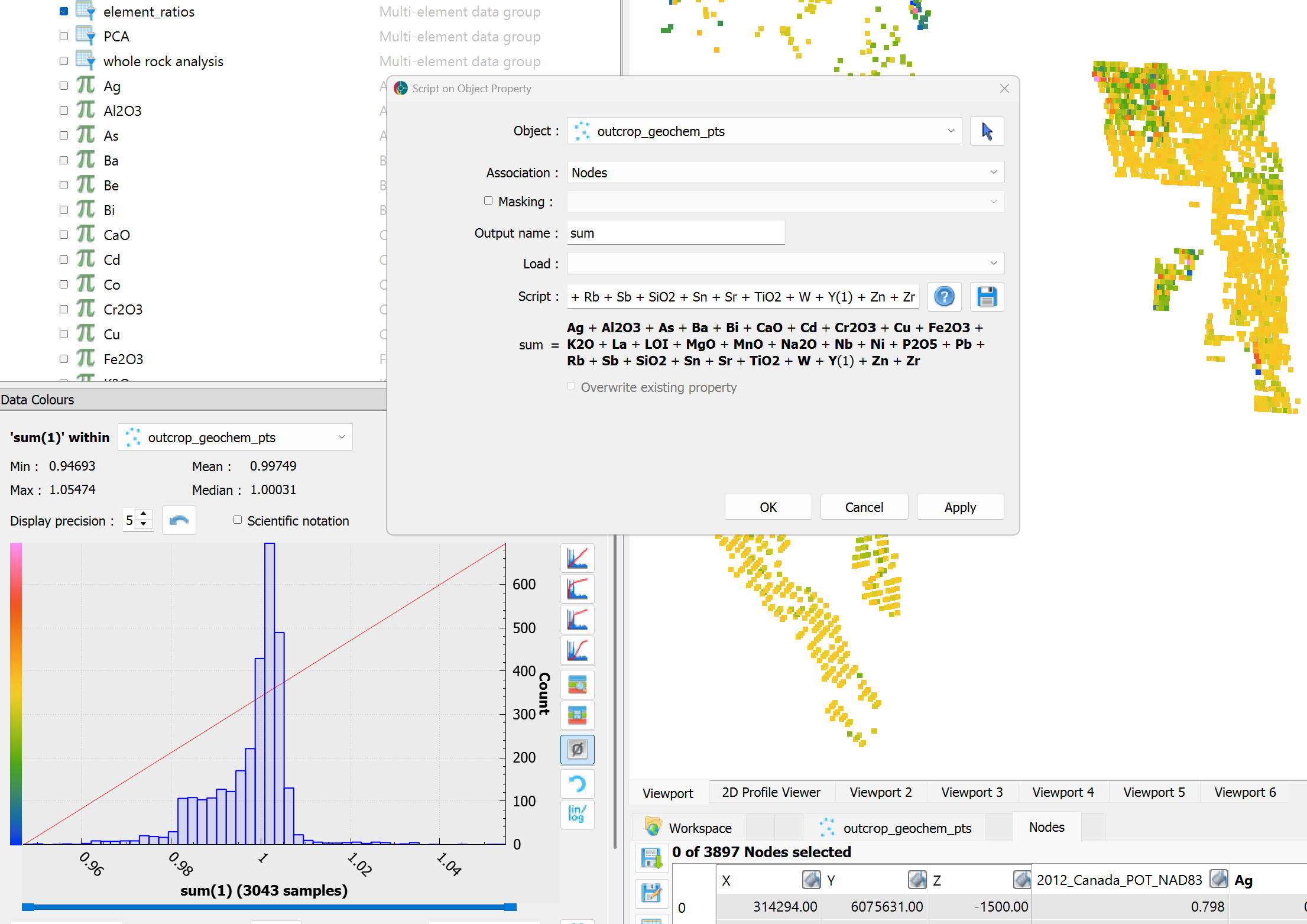
Fig. 16 Histogram of the sum of all compositional values per sample, confirming closure to 1 after unit conversion.

Note

Verify that all samples sum to 1 (or very close to 1) before proceeding. Significant deviations may indicate missing elements or unit conversion errors.

Centered Log-Ratio

Compositional data are subject to the closure effect: because all components sum to a constant, the variables are not statistically independent, which distorts distances, correlations, and variance. The Centered Log-Ratio (CLR) transformation addresses this by mapping the data into an unconstrained real space where standard multivariate methods can be applied reliably.

The CLR of a composition \(\mathbf{x} = (x_1, \ldots, x_D)\) is defined as:

\[\text{CLR}(x_i) = \ln\left(\frac{x_i}{g(\mathbf{x})}\right), \quad i = 1, \ldots, D\]

where \(g(\mathbf{x}) = \left(\prod_{i=1}^{D} x_i\right)^{1/D}\) is the geometric mean of the composition. This transformation removes the artificial negative correlations introduced by closure and places all elements on an equal footing regardless of their original magnitude.

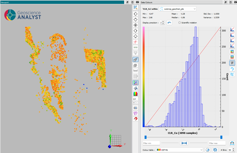
Fig. 17 CLR-transformed values for selected elements, illustrating the spread and symmetry achieved after transformation.

See the CLR application documentation for full details on the interface and usage.

Dimensionality Reduction with PCA

After CLR transformation, whole-rock geochemical datasets typically contain many correlated variables. Principal Component Analysis (PCA) is applied to reduce dimensionality while retaining the principal axes of geochemical variation.

PCA identifies linear combinations of the CLR-transformed elements that explain the maximum variance. Retaining the first few principal components (PCs) compresses the dataset while preserving the major geochemical trends needed for clustering.

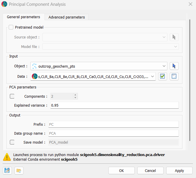
Fig. 18 Biplot of the first two principal components, coloured by sample location. PC1 and PC2 together explain the dominant geochemical variance in the dataset.

Refer to the PCA application documentation for details on interface options such as the number of components and explained variance threshold.

Self-Organizing Map Clustering

The PCA scores (or the full CLR-transformed dataset) are passed to the Self-Organizing Map (SOM) clustering algorithm. SOM projects the high-dimensional geochemical data onto a 2D grid of nodes while preserving the topological structure of the data. Each node is then assigned a cluster label, and every sample is associated with its closest node.

Once clustering is complete, the cluster labels are visualized back in geographic space. Samples belonging to the same SOM cluster share a common geochemical signature and tend to occur in spatially coherent domains, reflecting underlying lithological or alteration controls. 3 main distincstregions

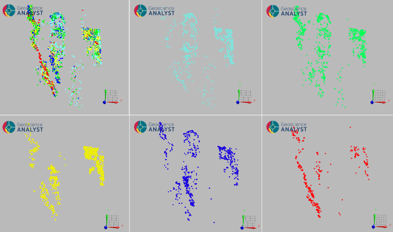
Fig. 19 Map of sample locations coloured by SOM cluster. Spatially coherent groupings suggest geochemical domains linked to distinct rock types or hydrothermal alteration zones.

See the SOM Clustering documentation for full interface details and advanced parameters.

Spatial Interpolation

Once geochemical domains are identified, spatial interpolation is used to project the data onto a continuous grid, enabling map-scale visualisation and spatial analysis. Interpolated maps facilitate the comparison of elemental distributions across the study area, the identification of spatial trends, and the integration with other spatial datasets such as geophysics or geology.

We are interested in comparing different interpolation methods to understand how they capture the spatial structure of the geochemical data. The methods compared in this study include:

• Neural kriging: A machine learning-based geostatistical method that models spatial autocorrelation and can incorporate secondary data.

• RBF interpolation interpolation: A smooth, deterministic method that fits a surface through the data points using radial basis functions.

• Inverse distance weighting (IDW): A simple method that estimates values based on the inverse of the distance to nearby samples, without accounting for spatial anisotropy - available with ANALYST.

• Multi-trending interpolation: A method that captures sharp contrasts along complex structural trends, often used in geological contexts - available with ANALYST.

Fig. 20 Comparison of interpolation methods applied to (A) CLR-transformed CaO values: (B) Neural kriging, (C) Neural kriging with secondary data, (D) RBF interpolation from grid search optimisation, (E) inverse distance and (F) multi-trending interpolation.

Results obtained with the neural kriging method reproduce the NNW–SSE anisotropy visible in the raw data. When secondary data are added, the result is unchanged, confirming that the model identified the covariate as non-informative for this dataset. RBF produces the smoothest surface insensitive to short-range variability. IDW lacks directional sensitivity and generates isotropic halos. Finally, the multi-trending captures sharp lateral contrasts.

Summary

Selecting an appropriate griding method depends on the geological context, data density, and interpretation objectives. Kriging-based methods are generally more appropriate when structural anisotropy is expected. RBF and IDW are parameter-light alternatives suited to reconnaissance datasets. Multi-trending is relevant when sharp geochemical contrasts are anticipated. Regardless of the method, cross-validation against held-out samples is required to assess predictive performance objectively. The six results shown here should be read as complementary spatial views of the same dataset, each sensitive to different aspects of its structure.