Geophysical Anomalies as Predictors for Copper Mineralization

This case study demonstrates a mineral prospectivity workflow that uses geophysical domain segmentation, proximity feature extraction, and spatial association analysis to identify geophysical signatures correlating with known copper indices. Two regional airborne and ground geophysical datasets are transformed into interpretable distance features, which are then evaluated against copper occurrences using a weight of evidence approach.

The QUEST-South Project Area

The QUEST-South project covers a 130 000 km² region in the southern interior of British Columbia. This area spans the highly prospective Quesnel terrane, a geological belt known for hosting major porphyry copper deposits. Because thick layers of glacial till and sediment hide the bedrock, traditional surface exploration is difficult.

Available Datasets

The project relies on three primary layers of data to map the geology hidden beneath the surface:

• Gravimetric data: Airborne gravity data that measures variations in rock density. This reveals the shapes of deep-seated, buried igneous intrusions.

• Magnetic data: High-resolution aeromagnetic data that measures magnetic susceptibility. This maps out structural faults, geological boundaries, and zones of hydrothermal alteration.

• Copper occurrences: Recorded data of known copper mineralisation, showings, and past-producing mines from MINFILE. These surface points anchor the geophysical data to proven copper-bearing systems.

The geophysical data were downloaded from the Geoscience BC - Quest South project page.

Note

[Downloaded here] the compilation geoh5 project containing the training data.

Input Geophysical Data

Two geophysical grids covering the study area are used as inputs.

The first is the Bouguer gravity anomaly with isostatic correction (QS-CBG-ISO). This layer represents the residual gravitational field after accounting for terrain, latitude, and long-wavelength isostatic compensation. It highlights density contrasts in the upper crust, which are relevant for identifying intrusive complexes and structural corridors commonly associated with porphyry copper systems.

The second is the total magnetic intensity reduced to the pole and upward continued at 5000 m (RMI UC 5000 m). Reduction to magnetic inclination removes the dependence of magnetic anomaly shape on latitude and field inclination, centering anomalies over their sources. Upward continuation at 5000 m suppresses high-frequency shallow noise and emphasizes deeper, regional magnetic bodies, typically magnetite-bearing intrusions that are spatially associated with copper-bearing magmatic systems.

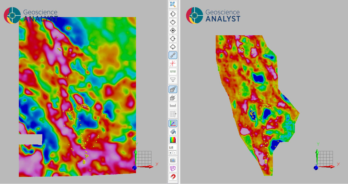
Fig. 21 Bouguer gravity anomaly with isostatic correction (left) and total magnetic intensity reduced to the pole, upward continued at 5000 m (right), covering the study area; the copper indices used as target occurrences are overlaid as yellow points.

Geophysical Domain Segmentation

The two geophysical grids are jointly segmented into seven spatially coherent domains using the 2D Grid Domains Segmentation (SLIC) application. SLIC groups neighbouring grid cells that share similar geophysical signatures across both inputs, producing compact, interpretable regions that capture the dominant geophysical character of the survey area.

The clustering detail parameter was set to 0.6. This parameter controls the reconstruction penalty used to determine the optimal number of clusters: higher values favour a finer partition with more clusters, while lower values (like the one used, 0.6) impose a stronger penalty on complexity and yield a coarser, more generalised segmentation. the present setting leads to seven domains, presented in the figure below.

The resulting seven domains partition the study area into units reflecting distinct combinations of density and magnetic response. These domains serve as the categorical layer on which subsequent distance features are computed.

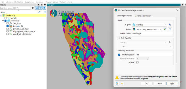
Fig. 22 Seven geophysical domains produced by SLIC segmentation of the combined gravity and magnetic grids. Each colour corresponds to one domain.

Distance Feature Extraction

The Distance to Categories application is applied to the seven-domain segmentation. For each location in the prediction grid, the Euclidean distance to the nearest cell belonging to each domain is computed, producing seven distance properties (one per unit).

These distance properties encode the spatial proximity of every grid cell to each geophysical domain and form the feature set used in the subsequent association analysis.

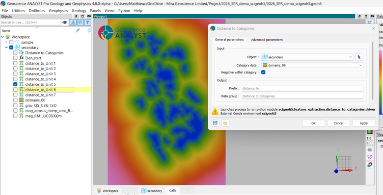
Fig. 23 Distance to each of the seven geophysical domains, computed across the prediction grid. Warmer colours indicate greater distance from the respective domain.

Spatial Clustering for Train–Test Split

Before running the association analysis, the copper indices are partitioned into spatially coherent training and test sets using the DBSCAN Clustering application. The algorithm is applied to the point locations with a distance (epsilon) of 15 000 m, producing spatial clusters that group nearby occurrences together.

The resulting clusters are then projected onto the prediction grid. The easternmost cluster is held out as the test set, while the remaining clusters form the training set. This spatial split ensures that the model is evaluated on a geographically independent subset rather than on randomly scattered points that would be spatially correlated with the training data.

Fig. 24 DBSCAN spatial clusters projected onto the prediction grid. The eastern cluster (dark) is used as the test set; the remaining clusters constitute the training set.

Weight-of-Evidence Analysis

The Weight of Evidence (WoE) application is applied using the seven distance features as predictors and the training set of copper indices defined previously as the binary target. Each distance feature is discretised into three bins defined by two optimal thresholds, and a weight is assigned to each bin according to the degree to which its spatial distribution matches the distribution of copper occurrences.

Note

Areas with no-data values were excluded from the analysis by converting the grid to points and removing the points that fell outside the data coverage.

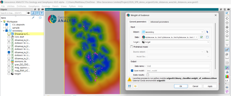
Fig. 25 Weight of evidence setup for the distance features.

The results are summarised in the table below, rows ordered by decreasing peak positive weight.

Table 1 Weight of evidence per distance feature and bin (training set only)

Feature	Threshold 1 (m)	Threshold 2 (m)	WoE bin 0 (< thr 1)	WoE bin 1 (thr 1 to thr 2)	WoE bin 2 (> thr 2)
Distance to Unit 4	−2 000	20 502	+1.26	+0.12	−0.90
Distance to Unit 7	4 717	12 918	−0.82	−0.31	+0.91
Distance to Unit 2	6 042	13 997	−0.35	+0.67	−1.06
Distance to Unit 6	4 497	18 032	−1.20	+0.15	+0.59
Distance to Unit 1	2 500	16 229	−0.35	+0.57	−1.18
Distance to Unit 5	11 308	15 635	+0.12	−1.80	+0.20
Distance to Unit 3	9 549	20 314	+0.16	−0.08	−0.57

The results are described below in decreasing order of peak WoE.

Unit 4 (gravity +14.67 mGal, magnetic +287.4 nT) shows the strongest positive proximity association (bin 0 WoE = +1.26), with a negative first threshold indicating that nearly all training points fall within the domain boundary. The weight decreases at intermediate distances and turns negative beyond 20 502 m.

Unit 7 (gravity +10.65 mGal, magnetic +0.1 nT) exhibits its peak positive weight in the far bin (bin 2 WoE = +0.91), indicating that copper indices in the training area tend to occur at distances greater than ~12 900 m from this domain rather than near it.

Unit 2 (gravity +5.94 mGal, magnetic +117.2 nT) has its peak weight in the intermediate bin (bin 1 WoE = +0.67), suggesting an optimal association at distances between ~6 000 m and ~14 000 m.

Unit 6 (gravity +2.47 mGal, magnetic −30.4 nT) follows a similar distal pattern, with negative proximity weight (bin 0 WoE = −1.20) and a positive far-distance weight (bin 2 WoE = +0.59), indicating that training occurrences are preferentially located away from this domain.

Unit 1 (gravity +2.00 mGal, magnetic +229.9 nT) peaks at intermediate distance (bin 1 WoE = +0.57) and is strongly negative beyond 16 229 m, suggesting a focused association at moderate proximity.

Unit 5 (gravity −8.01 mGal, magnetic +51.4 nT) shows a weak proximal weight (+0.12) and a strongly negative intermediate bin (−1.80), with a slight positive rebound at greater distances.

Unit 3 (gravity +16.58 mGal, magnetic +129.4 nT) has only weak associations across all bins, with its highest weight in the proximal bin (+0.16) and decreasing values further away.

In synthesis, mineralisation appears to concentrate near dense, strongly magnetic intrusive bodies (Unit 4) and at distance from demagnetised or non-magnetic domains (Units 6 and 7), a pattern consistent with copper deposits controlled by the margins of oxidised, magnetite-stable magmatic systems.

Prospectivity Results

The combined WoE score reveals a dominant N–S trending corridor of elevated prospectivity, with a secondary E–W extension at the latitude of the highly mineralised testing area. The model was trained so that a score of zero represents the threshold between mineralised and non-mineralised conditions.

Fig. 26 Weight of evidence total score across the study area. The testing area (eastern cluster) is outlined by the green dotted boundary; copper indices are overlaid as points.

Copper indices within the testing area fall into slightly negative WoE zones. Although these values are not positive, they remain close to zero compared to the regional background, which drops below −2. This contrast indicates that the spatial relationships identified by the WoE model on the training set still highlight geophysically meaningful trends in the independent test area.

A few target points lie outside the near-zero or positive WoE corridors altogether. These occurrences may be related to mineralising processes that are not captured by the geophysical distance features used here, suggesting that complementary predictors would be needed to account for the full range of copper deposit styles in the study area.

Note

The distance features are derived from the same geophysical fields and are therefore correlated. The conditional independence assumption of the WoE framework is not satisfied; however, in geological applications input variables are rarely truly independent, so the combined score should be treated as a qualitative ranking rather than a calibrated probability.

Note

Mineralisation may not occur at the apex of the causative system. The regional gravity anomaly integrates density contrasts over depth, introducing a lateral shift between the 3-D source and its 2-D map projection. This can produce spatial interference between overlapping sources, potentially displacing predicted prospectivity corridors relative to true deposit locations.