2D Grid Domains Segmentation

The 2D grid domains segmentation application provides tools to partition 2D gridded datasets (geophysics, geochemistry, radiometric, etc.) into meaningful regions, based on their properties and spatial relationships. Segmentation enables the identification of areas sharing similar geophysical characteristics, supporting interpretation and analysis.

The workflow begins by generating a simplified representation of the data using the SLIC algorithm, which produces superpixels that capture local patterns and boundaries. These superpixels serve as the basis for further segmentation steps.

The application, presented in the figure above, offers three main functionalities: offers three main functionalities:

• Cluster regions based on values: Group superpixels according to their average property values

• Cluster regions based on spatial continuity and values: Merge superpixels considering both their values and spatial adjacency for more geologically meaningful domains.

• Use control points to spread labels: Assign labels to selected superpixels and propagate them to neighboring regions, enabling semi-automatic domain definition.

Note

The segmentation results produced by this application are based solely on mathematical and statistical criteria. They do not constitute a geological interpretation, but rather provide regions defined by objective, algorithmic logic. Further expert analysis is required to assign geological meaning to the segmented domains and adjust the regions accordingly.

Interface

General Parameters

The main parameters controlling the 2D grid domains segmentation application are shown in the figure below.

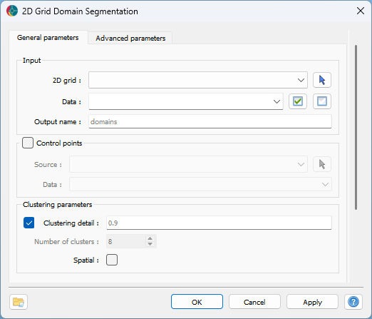
The options are described as follows:

Objects Selection

• Client: The object containing the data to segment.

• Data: The data properties used for segmentation. Multiple Float properties can be selected.

• Property group (optional): Alternatively, select a group of related data properties for segmentation. If used, individual property selection is disabled.

Control Points

• Source (optional): The object containing control points to guide the segmentation. If specified, the segmentation will use these points to propagate labels across the dataset.

• Data (optional): The data property associated with the control points. If not specified, the first available property will be used.

Clustering Parameters

• Clustering detail (default: 0.9): Find the optimal number of clusters based on the reconstruction penalty. Higher values result in more clusters, while lower values yield fewer clusters.

• Number of clusters (optional): The number of clusters to generate. Activate Clustering detail to automatically determine the optimal number of clusters based on the data.

• Spatial: Enable spatially-aware graph-based clustering for more geologically meaningful domains.

Output Names

• Output name: The name of the created segmentation output. If not specified, the default name will be “Geophysical Domains”.

Optional Parameters

Advanced controls for the segmentation process are available as optional parameters.

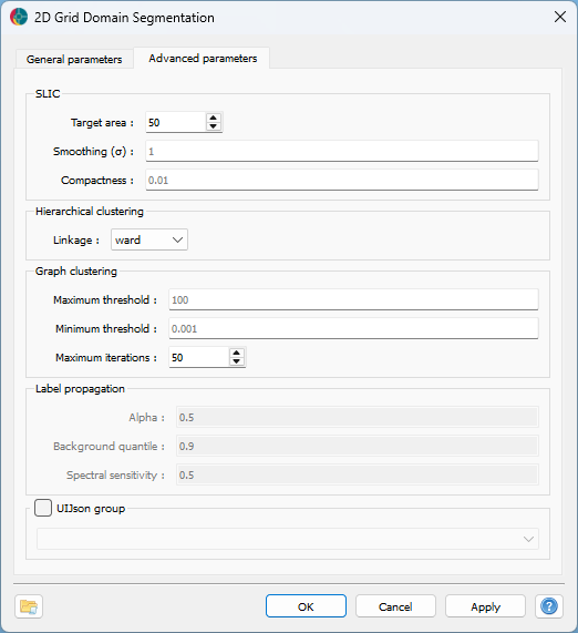
SLIC Parameters

Parameters passed on to the skimage.segmentation.slic algorithm.

• Target area (default = 50): Target area (in number of pixels) for each superpixel.

• Smoothing (σ) (default = 1.0): Sigma used for Gaussian smoothing before segmentation.

• Compactness (default = 0.01): Compactness value for enforcing spatial regularity.

Hierarchical Clustering

• Linkage (default = “ward”): Linkage method used for hierarchical clustering.

Graph Clustering

• Maximum threshold (default = 100): Maximum threshold for graph-based merging.

• Minimum threshold (default = 0.001): Minimum threshold for graph-based merging.

• Maximum iterations (default = 50): Maximum number of iterations for graph clustering threshold search.

Label Propagation

• Alpha (default = 0.5): Controls the extent of label propagation during segmentation. Higher values allow labels to spread more across regions.

• Background quantile (default = 0.9): Superior quantile distance value for background thresholding.

• Spectral sensitivity (default = 0.5): Controls how strongly feature differences affect label diffusion. Higher values make the algorithm more sensitive to feature differences, resulting in sharper boundaries.

Once the parameters are selected, press OK to run the segmentation and obtain results as shown in the first figure.

Results

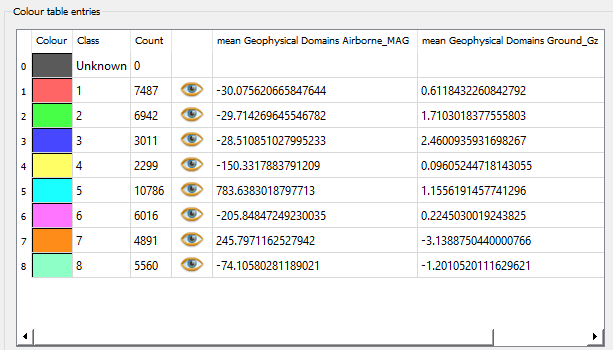
The results of the segmentation process are stored in the same object as the original data, with a new property named “Geophysical Domains” (or the specified output name). This property is a Referenced data representing the assigned domain for each superpixel or pixel in the dataset.

As presented in the figure below, the mean of the selected data properties is calculated for each domain, providing a summary of the geophysical characteristics within each segmented region.

Methodology

Before being sent to the clustering algorithms, the data undergoes a preprocessing step to normalize the values and create a mask that excludes invalid data. This processing step consists in applying a robust scaling tangent (RobustTanScaler) to the data, which is a robust scaling method that applies a tangent transformation to the data. This transformation is particularly useful for geophysical datasets, as it reduces the influence of outliers and extreme values, allowing for a more stable segmentation process.

SLIC super-pixels

The SLIC algorithm is used to divide a geophysical dataset into small, spatially coherent regions called superpixels. Each superpixel groups together neighboring cells or pixels that have similar property values, simplifying the dataset while preserving important boundaries and patterns. This initial segmentation provides a flexible foundation for further grouping and analysis.

Clustering

Once superpixels are generated, the next step is to group them into larger domains based on their values and spatial relationships. This can be done using various clustering methods, each with its own approach:

Hierarchical segmentation

After generating superpixels, the next step is to group them into larger, meaningful domains. Hierarchical clustering builds a “tree” based on the similarity of superpixel values. Superpixels that are most similar are merged first, and the process continues until all are grouped.

Graph segmentation

Alternatively, clustering can consider both the values and the spatial relationships between superpixels. In this approach, a graph is constructed where each superpixel is a node, and connections (edges) represent spatial and value-based similarity. Clusters are formed by merging connected superpixels, resulting in domains that are both similar in value and spatially continuous—better reflecting geological structures.

Clusters vs. reconstruction

Users can choose the number of clusters based on their analysis needs. More clusters provide finer detail, while fewer clusters yield broader regions. The application allows users to specify a target number of clusters or automatically determine it based on the data.

Users can also evaluate the clustering detail by adjusting the “clustering detail” parameter. This parameter helps find the optimal number of clusters by balancing detail and simplicity. It does so by evaluating how well the clusters represent the original data, known as the “reconstruction penalty.” As the number of clusters increases, the representation improves but becomes more complex. The goal is to minimize this penalty while avoiding unnecessary complexity.

Control points

In some cases, users may want to guide the segmentation using control points. By assigning labels to specific superpixels, these labels can be propagated to neighboring regions based on similarity and spatial proximity, using a graph-based approach. This allows users to define key regions of interest and ensure that the segmentation aligns with geological expectations. This semi-automatic approach allows experts to incorporate their knowledge and refine the segmentation to match geological expectations.

Example

The following examples demonstrate how to use the 2D grid domains segmentation application in different scenarios. Each tutorial is illustrated with an animation showing the workflow and results.

Spatial Graph Clustering (Automatic Number of Clusters)

This example shows how to segment a dataset using spatially-aware graph clustering, where the optimal number of clusters is determined automatically based on the reconstruction penalty.

• Open the segmentation application.

• Select the object and data properties to segment.

• Enable the Spatial option in clustering parameters.

• Run the application to generate domains that are both spatially coherent and similar in value.

Hierarchical Clustering (Fixed Number of Clusters)

This example demonstrates hierarchical clustering, where the user specifies the desired number of clusters.

• Open the segmentation application.

• Select the object and data properties to segment.

• Set the Number of clusters to the desired value.

• Run the application to group regions based on their property values.

Segmentation with Control Points

This example illustrates how to guide the segmentation using control points.

• Open the segmentation application.

• Select the object and data properties to segment.

• In the Control Points section, select the object containing your control points and the associated data.

• Run the application to propagate labels from the control points, refining the segmentation according to expert knowledge.