Neural Kriging

Neural Kriging is an interpolation method that estimates values at unknown locations based on surrounding data points. It is inspired by traditional geostatistical methods like inverse distance weighting (IDW) and kriging. It incorporates a trainable neural network to enhance predictions.

A key feature of Neural Kriging is that users do not need to define interpolation parameters. The model automatically learns the optimal distance weighting, rotation, and influence of secondary variables based on the dataset. This makes it an adaptable tool for geologists looking to model spatial data without extensive parameter tuning. This automated learning approach is particularly useful in geosciences, where geological and geochemical patterns are often nonlinear and influenced by multiple factors.

Interface

The application only requires the data to interpolate and the object where the interpolation will be saved. The interface is presented in the Fig. 2.

Fig. 2 Neural Kriging Interpolation main interface

Input

• Source: The object containing the data to use for the interpolation.

• Pretrained model file (optional): If users have a pretrained model, they can load it here. It must be associated to the source object. The data the model was trained on must be present in the source object.

• Data: The primary data to interpolate.

• Destination: The object on which the data will be interpolated.

• Distance threshold: If activated, only points within the specified distance to source points will be interpolated.

Secondary data (optional)

If activated, users can include secondary data for the interpolation. The secondary data must be named the same in both the source and destination objects. The following options are available:

• Source: The secondary data from the source object.

• Destination: The secondary data from the destination object.

Output

• Name: The name of the output variable.

• Save model (optional): If activated, users have to define the name of the model to save in the source object.

• Uncertainty: If activated, along the interpolated values

  • the application will output each class probability for referenced data;

  • the application will output the uncertainty estimation for continuous data.

Advanced parameters

The application provides several advanced parameters to customize the interpolation process. The Fig. 3 shows the available options. The default values should work well for most cases.

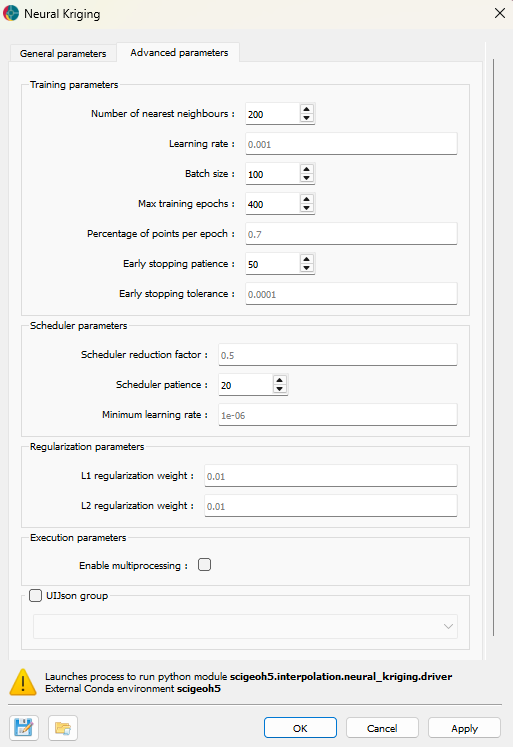
Fig. 3 Neural Kriging Interpolation advanced parameters interface

Training parameters

• Number of nearest neighbors: Specifies the number of closest data points used for interpolation. A higher number of neighbors smooths predictions but increases computation time, while a lower number preserves local variations but may introduce noise.

• Learning rate: Controls how quickly the model updates during training. A higher learning rate speeds up convergence but risks instability, whereas a lower learning rate ensures more gradual, stable learning at the cost of longer training times. If the interpolation converge into a non-optimal solution, users can try to reduce the learning rate.

• Batch size: Defines the number of data points processed at once during training. Larger batch sizes improve computational efficiency but may generalize poorly, while smaller batch sizes capture finer details but require more iterations.

• Max training epochs: The maximum number of times the model processes the dataset. More epochs allow for better learning but increase runtime. Early stopping mechanisms prevent unnecessary computations when the model stops improving.

• Percentage of points per epoch: Specifies the fraction of available data used in each training epoch. A higher percentage stabilizes training but increases computation time, while a lower percentage introduces more randomness, potentially enhancing generalization.

• Early stopping patience: Defines how many epochs the model will continue training without improvement before stopping. A higher patience prevents premature termination but may lead to overfitting.

• Early stopping tolerance: Sets the minimum improvement threshold to consider the model as having improved. A smaller tolerance makes the model more sensitive to minor improvements, while a larger tolerance focuses on significant changes.

Scheduler parameters

• Scheduler reduction factor: Determines the step size for reducing the learning rate when training stagnates. A lower factor results in smaller adjustments, while a higher factor decreases learning rate more aggressively.

• Scheduler patience: Specifies the number of epochs without improvement before reducing the learning rate. A higher patience delays learning rate adjustments, while a lower patience makes adjustments more frequent.

• Minimum learning rate: Defines the lowest value the learning rate can reach during training, ensuring that training does not completely stop even after multiple reductions.

Regularization parameters

• L1 regularization weight: Encourages sparsity in the model by penalizing large weights. A higher L1 weight reduces complexity but may remove useful patterns, while a lower weight allows for more flexibility.

• L2 regularization weight: Prevents large weight values, improving generalization. A higher L2 weight enhances stability but may underfit data, while a lower weight provides more adaptability.

Execution parameters

• Enable multiprocessing: Allows parallel processing to speed up training. Enabling this feature reduces computation time but requires more system resources. The multiprocess will be run on half the cpu cores available.

Methodology

Interpolation

As presented in the Fig. 4, this application aims to find the optimal weights of surrounding points to predict the value at a target location. This section explains how those weights are calculated.

Fig. 4 Interpolating a point by weighting surrounding points.

Neural Kriging follows a step-by-step process to calculate interpolated values:

1. Compute the distance to neighboring points in 3D space (\((x, y, z)\)).

   \[\Delta_{\text{distance}} = (x_{\text{point}} - x_{\text{neighbor}}, y_{\text{point}} - y_{\text{neighbor}}, z_{\text{point}} - z_{\text{neighbor}})\]

2. Apply a trainable transformation matrix to adjust for anisotropy.

   \[\Delta_{\text{rotated}} = \mathbf{R} \cdot \Delta_{\text{distance}}\]

This transformation matrix (\(\mathbf{R}\)) enables the model to learn the optimal linear transformations of the space, such as anisotropy, rotation, and shearing, as illustrated in the Fig. 5. This process allows subsequent steps to be performed in an isotropic space.

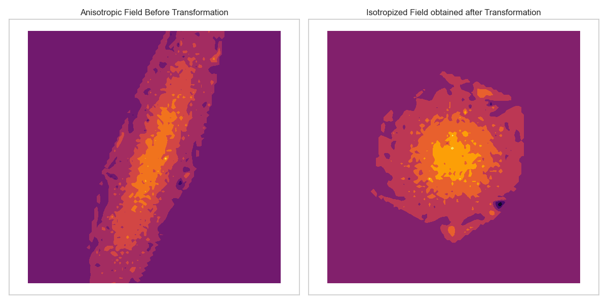
Fig. 5 Deformation of space to account for anisotropy.

3. For each point \(i\) compute interpolation weight (\(w\)) using the Euclidean norm of the rotated distance vector and trainable range and nugget parameters:

   \[w_i = \frac{1}{\textit{nugget} + \|\Delta_{\text{rotated}}\|_2^{\textit{range}}}\]

This function allows to assigned weights based on distance, similar to IDW. It also include the concept of kriging : a range parameter controls how quickly weights decrease with distance, while the nugget parameter prevents weights from becoming excessively large for very close points, as illustrated in Fig. 6.

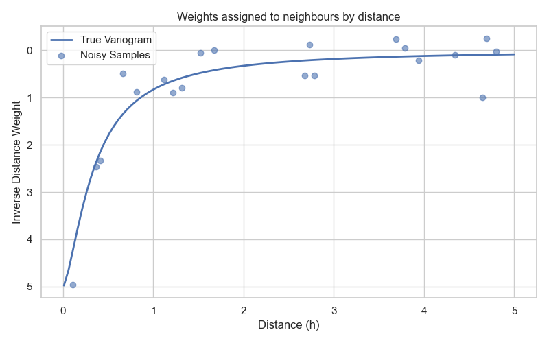
Fig. 6 Exponential function defining the weights based on distance.

4. Modify the weights using a trainable neural network (one layer only) that incorporates secondary variables. This difference between the predicted and actual secondary variable values (\(\Delta_{\text{secondary variables}}\)) is used as input to the neural network:

   \[w_i = w_i \times \textit{NeuralNetwork}(\Delta_{\text{secondary variables}})\]

The neural network determines a factor that modifies the weights. As illustrated in Fig. 7, if a secondary variable is positively correlated with the primary variable, the neural network increases the weights for points with similar secondary variable values. If the secondary variable is negatively correlated, it decreases the weights. This enables the model to adaptively adjust the influence of surrounding points based on additional information. If the secondary variables are not correlated with the primary variable, the neural network will learn to output a factor of 1, effectively leaving the weights unchanged. If no secondary variables are provided, this step is skipped.

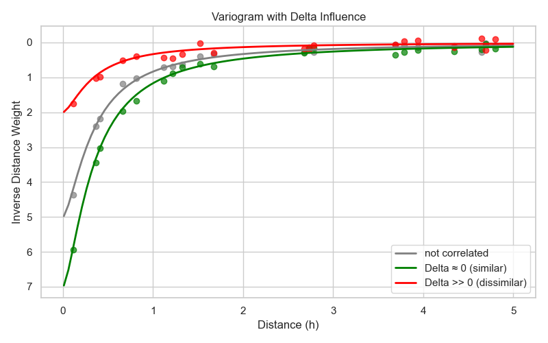
Fig. 7 Modification of weights based on secondary variables difference.

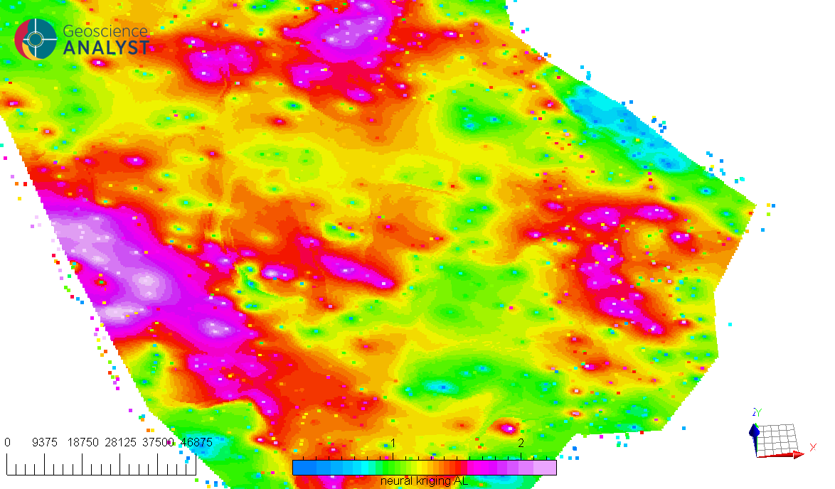
For examples, the Fig. 8 illustrates an interpolation (A) conducted with no secondary data. On this interpolation, a clear NW-SE anisotropy is visible. For comparison, the same interpolation is performed (B) but this time including a secondary variable (C) that is correlated with the primary variable. In this scenario, the model learns to increase the weights of points with similar secondary variable values, resulting in an interpolation deformed to align with the anomalies of the secondary variable.

Fig. 8 Example of the influence of secondary variables on the interpolation; (A) interpolation without secondary variable, (B) interpolation with secondary variable, (C) the “interpreted basement domains anomalous apparent susceptibility” used as secondary variable.

5. Compute the final predicted value using a weighted sum:

   \[\hat{v} = \frac{\sum (w_i \times v_i)}{\sum (w_i)}\]

The final prediction uses the values of each surrounding point (\(v_i\)), weighted by the learned weights for each point found previously, to estimate the value at the target location. During training, the target location is known, and the model is trained to minimize the difference between the predicted value \(\hat{v}\) and the actual value at that location, as shown in the Fig. 9. Training is performed on a subset of the data (Percentage of points per epoch option), and the model is optimized to generalize well to unseen locations.

Fig. 9 Training the model to minimize the error between predicted and actual values.

Between each training epoch, the model’s performance is evaluated. Using all available points, the model predicts values and computes the RMSE (Root Mean Square Error). If the RMSE does not improve for a specified number of epochs (the early stopping patience option), the learning rate is reduced by a factor defined by the scheduler reduction factor option. This adaptive learning rate strategy helps the model converge more effectively. If the RMSE still does not improve after several reductions (the scheduler patience option), the training stops. This saves computation time.

Because the input data are scaled, the RMSE values can be interpreted as a fraction of the data standard deviation. A value of 1 indicates that the RMSE is equal to the standard deviation of the data, while a value of 0.1 indicates that the RMSE is 10% of the standard deviation. This value is saved in the metadata of the source object.

Uncertainty estimation

If the Uncertainty option is activated, the application provides uncertainty estimates for the interpolated values.

Referenced Data

If the Data used for interpolation are referenced data, the application outputs a probability for each category at every interpolated point. During training, the model learns one output channel per category. Each channel estimates the relative weight of its category based on the surrounding data points.

The final predicted category at a given location is obtained by selecting the category with the highest estimated weight. In this context, the output probabilities represent the model’s relative confidence for each category at that point.

Continuous Data

If the Data used for interpolation are continuous values, the uncertainty is defined as:

\[\sigma = \sqrt{\frac{\sum_i w_i \left( v_i - \hat{v} \right)^2}{\sum_i w_i}}\]

This quantity measures how consistent the surrounding data values are with the predicted value \(\hat{v}\). Each neighboring value \(v_i\) contributes to the uncertainty according to its weight ratio where \(w_i\) is the interpolation weight of neighboring point i. The weight ratio therefore reflects the relative influence of each neighbor on the interpolation. If the most influential neighboring points have similar values, the uncertainty is low; if they differ significantly, the uncertainty increases.

This uncertainty reflects both local data variability and the capacity of the spatial model to explain it through the computed interpolation weights. It therefore provides a data-driven measure of confidence in the predicted value, based on how well the surrounding observations are reconciled by the spatial model.

As the data are normalized during processing, the uncertainty values are expressed in normalized units. An uncertainty value close to 1 indicates that the local variability around the prediction is comparable to the overall variability of the dataset, while a value close to 0.1 indicates much lower local variability relative to the global scale.

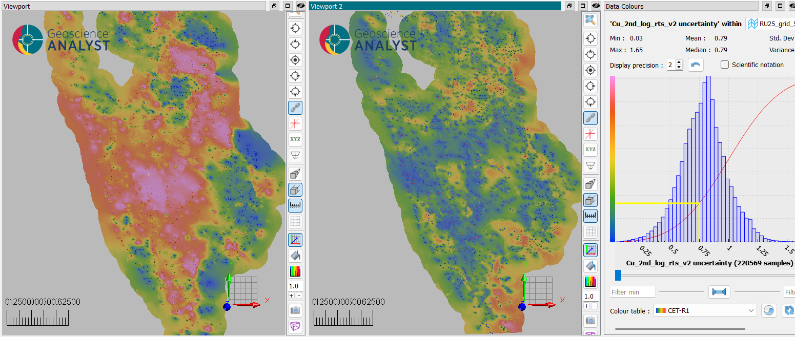
Fig. 10 Illustration of uncertainty estimation (viewport 2) of an interpolation (viewport 1) based on surrounding data variability.

Pre-processing

The following pre-processing steps are performed by the function before applying the interpolation:

• Filtering points:

  • Only points containing valid values are kept for interpolation.

  • In the case of secondary variables, all points containing “no-data” values will be excluded.

• Secondary variable normalization:

  • Secondary variables are normalized by subtracting their mean and dividing by their standard deviation.

• Normalization of the primary data:

  • The data to be interpolated is normalized by subtracting its mean and dividing by its standard deviation.

  • After interpolation, the results are transformed back to the original scale by multiplying by the variance and adding the mean.

• Distance-based filtering (optional):

  • If activated, data further than a specified distance from the points to interpolate will not be interpolated.

Note

The interpolation result depends, among other factors, on the distribution of the input data values, and strongly skewed distributions or long tails may bias the prediction. Appropriate preprocessing can improve model stability and accuracy in the chosen data representation, as no automatic distribution correction is applied.

Tutorial

The following animated image presents a tutorial on how to use the Neural Kriging Interpolation application.

• Select the object containing the data to interpolate.

• Select the data to be interpolated.

• Select the object to project the interpolated data onto.

• (Optional) Define the name of the output object.

• (Optional) Select the secondary data for the source object.

• (Optional) Select the secondary data for the destination object.

• (Optional) Define a distance threshold to limit the interpolation range.

• Run the application.

• Inspect the results.