Principal Component Analysis
Principal Component Analysis (PCA) is a dimensionality reduction technique that simplifies complex datasets by identifying principal components—directions of maximum variance in the data. These components are linear combinations of the original properties, ranked by their importance in explaining the variance.
For example, PCA can highlight geochemical trends from core samples in magmatic settings. A principal component with high silica can indicate samples of granitic compositions, while another component rich in iron may indicate magma mixing. Various components combined can help geologists identify magmatic processes or compositional patterns.
Pre-processing
Before proceeding with the PCA, the data are normalized if the option is activated. Normalization is done by subtracting the mean and dividing it by the standard deviation of each property.
Data points containing any properties with no-data value are excluded from the PCA.
Warning
If all points contain one no-data value, PCA cannot be performed. There should be at least as many valid data points (no empty data) as there are properties.
Interface
General parameters
The general parameters controlling the Principal Component Analysis are shown in the figure below.
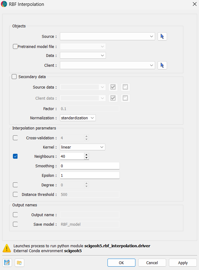
The options are described as follows:
Pretrained model
Source object: The object containing the weights of a pre-trained PCA model. If a model is provided, the application will use the weights to transform the data.
Model file (optional): If users have a pretrained model, they can load it here. The data the model was trained on must be present in the source object.
Input
Object: The object containing the data to be analyzed.
Data: The data to be analyzed. Users can select as many
Floatdata properties as desired.
PCA parameters
Components (optional): The number of principal components to compute. Must be an integer greater than 0.
Explained variance (default = 0.8): The total variance to be explained by the principal components. This must be a float between 0 and 1, representing the percentage of total variance. This option is used only if Number of components is not set.
Output
Prefix: The prefix added to each principal component name in the output group.
Data group: The name of the output group.
Save model (optional): If activated, users have to define the name of the model to save in the source object.
Advanced parameters
Advanced controls on the Scikit-Learn PCA algorithm are available as advanced parameters, as shown in the figure below.
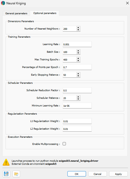
Standardize (optional): If checked, the data will be normalized before performing Principal Component Analysis (PCA).
Whiten (optional): If checked, the components are scaled to unit variance. Whitening removes correlations between features but may reduce interpretability.
SVD solver (default=’auto’): Determines the algorithm used for computing the principal components. Options include:
auto: Chooses the solver based on data size.full: Uses a full Singular Value Decomposition (SVD) approach.arpack: Uses a truncated SVD.randomized: Uses a fast, approximate randomized SVD.
Tolerance (default=0.0): The tolerance for the singular values computed during the SVD.
Iterated power (optional, default=0): The number of iterations for the randomized SVD solver.
Oversamples (default=10): The number of additional random vectors to sample the range of the matrix.
Power iteration normalizer (default=’auto’): The method to normalize the power iterations. Options include:
auto: Chooses the normalizer based on the solver.QR: Uses the QR decomposition (a mathematical decomposition method for matrices).LU: Uses the LU decomposition (another method for matrix factorization).
Random state (optional): Controls the randomness of the solver when svd_solver =
randomized. Pass an integer for reproducibility.
Once the parameters are selected, press OK to run the analysis.
Results
The application create a new group, as presented in the figure below. This group is named as defined in the Output name parameter and the new data created are name “Output name” + PC_n where n is the number of the component.
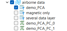
In the metadata, for each Principal Component axis, the coefficients of the linear combination of the original properties and the explained variance ratio for each principal component are stored.
If the option is activated, the saved weights are stored under the Object as “defined name” + .pkl.
Tutorial
The following animated image presents a tutorial on how to use the PCA application.
Open the application.
Select the object containing the data.
Select the data to be analyzed.
Define the number of components or the explained variance.
(optional) Choose the name to save the model.
Run the application.
Inspect the computed principal components.
To run a pretrained model
Select the object containing the data.
Select the data to be analyzed.
Select the object containing the weights.
Select the pretrained model file.
Run the application.