Weight of Evidence
Weight of Evidence (WoE) is a binary classification technique commonly used in mineral prospectivity mapping and risk analysis. It transforms input predictor variables into categorical bins and assigns each bin a weight. These weights reflect the degree to which the presence (or absence) of a variable correlates with known target occurrences.

In practice, the weight for each bin is computed based on the ratio of the proportion of targets within the bin to the global proportion of targets. This allows WoE to quantify spatial associations between geological properties and known mineralization. The method is data-driven, interpretable, and well-suited for integrating multiple geological layers in a simplistic mineral exploration workflows.
Interface
At a minimum, the application requires the selection of an object, property data to analyze and a binary target label (True or False mask). The interface is presented in the figure below.
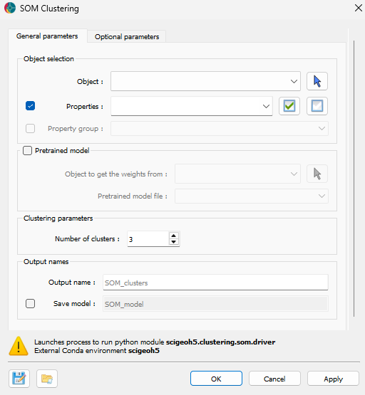
Pretrained model (optional)
Source object (optional): Allows users to use an existing WoE model. The object and file associated with the pretrained model can be specified.
Model file (optional): The file containing the weights of the pretrained model to apply to the data.
Input
Object: The object containing the data to analyze. This is the primary input for the WoE calculation.
Data (optional): The input data for the WoE calculation. Users can select multiple properties associated with the object.
Target: The binary target variable for the WoE calculation. This defines the classification target.
Output
Data name: The name for the resulting data with the WoE results.
Save model (optional): The name for the output file containing the WoE model. The file will be suffixed with
.xlsx.
Advanced parameters
The application provides several advanced parameters to customize the analysis process. The figure below shows the available options.
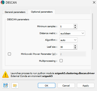
Output
Scale results: Whether to scale the results between 0 and 1.
Infer on no-data: If checked, the model will infer on points containing no data. If unchecked, these points will be ignored.
Training Parameters
Number of thresholds: The number of thresholds to use for the WoE calculation.
Output distribution: The distribution of the output. Options include
normaloruniform.Number of quantiles: The number of quantiles to use for the WoE calculation.
Random state (optional): A random seed for reproducibility.
Maximum iterations: The maximum number of iterations for optimization.
Tolerance: The tolerance for convergence in optimization.
Methodology
The WoE method quantifies the association between each class of a categorical variable and a binary target. It does so by comparing the proportion of positive targets within each class to the global proportion of positives across the dataset.
Mathematically, for each class \(i\), the WoE is computed as:
where:
\(P(T=1 \mid X=i)\) is the proportion of targets (\(T=1\)) in class \(i\)
\(P(T=1)\) is the global proportion of targets
The figure below below illustrates this concept using a categorical variable with three classes: A, B, and C. The histogram displays the frequency of each class, with overlaid pie charts representing the proportion of positive and negative targets. The computed WoE for each class is shown above the bars.
Negative WoE (e.g., category A): indicates that the class is less likely associated with the target than expected globally.
WoE near 0 (e.g., category B): indicates no strong relationship.
Positive WoE (e.g., category C): indicates that the class is more likely associated with the target than expected globally.

Fig. 11 Histogram of category frequencies for A, B, and C. Each bar includes a pie chart showing the proportion of positive vs. negative target values, with the computed WoE annotated above.
The same WoE logic applies to continuous variables. In this case, as presented in the figure below, the continuous predictor is discretized into bins using threshold values, and each bin is treated like a categorical class. For each bin, the proportion of positive targets is compared to the global proportion, and the corresponding WoE is computed.

Fig. 12 Histogram of a continuous variable segmented into bins using threshold values. Each bin is treated as a category. Pie charts show the proportion of positive vs. negative targets in each bin, with the corresponding WoE values annotated above.
In the present application, the thresholds are determined automatically during training using the scipy minimize scipy.optimize.minimize function with the Powell method, optimizing a balanced logistic loss.Users can subsquantly adjust the values of the thresholds or the associated weights manually by editing the output spreadsheet if needed.
Once the thresholds for continuous variables are determined and the WoE values are computed for all bins or categories, the model can be applied to new, unseen data. During inference, each input value—categorical or continuous—is mapped to its corresponding bin or class, and the associated WoE is assigned.
Note
When using WoE (especially with a limited number of thresholds ≤ 2), the model has such low complexity that the risk of overfitting is minimal. It is therefore acceptable to compute WoE values and apply them on the same dataset without separating training and inference phases.
Results
The results of the WoE methodology include both spatial outputs, as presented in the figure below, and tabular representations of the learned binning and WoE mappings.
Fig. 13 (Left) Spatial distribution of target occurrences (right) and the resulting Weight of Evidence values computed using a set of input properties.
These WoE values reflect the statistical association of each individual geological variables with the presence of targets. The final result, the sum of the WoE values across all input properties, give a score for each spatial location.
However, this score is not a probability score as each input variable is treated independently.
Saved weights
In addition to spatial results, the WoE processing exports a structured spreadsheet containing two key sheets (if the Save model option is enabled):
Those weights are the most important output of the WoE methodology, as they give a score of association for each data bin or category with respect to the target variable.
These scores provide an indication of association and are primarily useful for exploratory data analysis to identify potentially predictive features, rather than providing definitive statistical relationships.

Fig. 14 Example of the exported spreadsheet showing thresholds and WoE values for both continuous and categorical variables.
Thresholds_WoE
This sheet presents the binning configuration and computed WoE values for continuous properties. It includes the following columns:
feature_name: Name of the continuous property.
thresholds: The set of cut points (e.g.,thr_1,thr_2, …) used to define bins.Columns for each bin (e.g.,
woe_bin_0,woe_bin_1, …)
There is a row for each input property.
Referenced_WoE
This sheet contains WoE mappings for categorical features. It includes:
category_index: The unique class label for each category.Columns for each categorical properties, with WoE values indexed by the class.
Tutorial
The following tutorials demonstrate how to use the WoE application for both training a model and performing inference.
Training the Model
The following animated image shows how to train a WoE model:
Select the object containing the data to analyze.
Select the data to use for the WoE calculation.
(Optional) Define the name of the output object.
(Optional) Save the model by specifying a name for the output file.
Run the application to compute the WoE model.
Inspect the results.
Inference
The following animated image shows how to use a pretrained WoE model for inference:
A spreadsheet containing the pretrained model contains two tabs: one for the continuous properties and one for the categorical properties; it must be present on an object.
Open the WoE application interface.
Select the object containing the data to compute the WoE.
Select the object containing the pretrained model file.
Select the pretrained model file from the object (the file must be in
.xlsxformat).(Optional) Define the name of the output object.
Run the application to perform inference.
Inspect the results.