Random Forest

Random Forest is a supervised machine learning algorithm that learns to assign a category label to each data point by training a large number of simple decision trees, then combining their individual votes to produce a final prediction.

Each tree in the forest is trained on a slightly different random sample of the data and considers only a random subset of the input features at each decision step. This diversity means the trees will disagree on borderline cases, and the final label is determined by which class receives the most votes across all trees. Because the model is built from many independent trees rather than a single complex rule, it tends to be more robust than a single decision tree, though it remains sensitive to the quality and representativeness of the training data, and can still overfit or underfit (see the Methodology section).

In geosciences, Random Forest can be used to predict categorical properties across an entire dataset from a limited set of labelled samples — for example, classifying lithological units from geochemical or geophysical measurements, mapping alteration zones, or predicting rock types in undrilled volumes.

Note

• The Random Forest application requires a categorical target property with at least two non-zero class labels. Regression targets are not supported.

• Random Forest should be used as part of a broader modelling workflow, and not as a standalone application, or the model is likely to suffer from overfitting or underfitting.

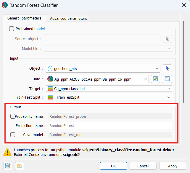
Interface

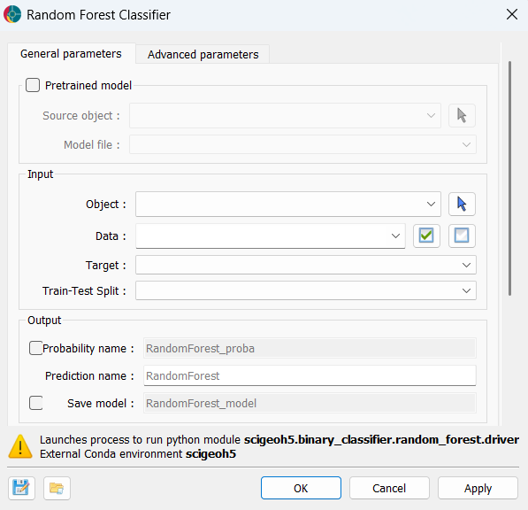
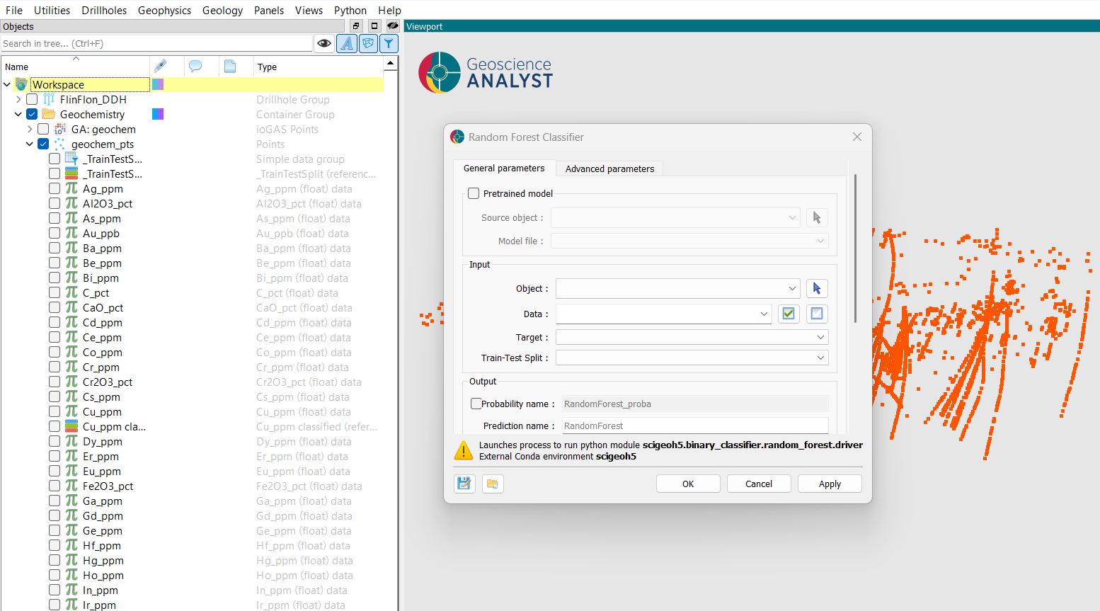
At a minimum, the application requires the selection of an object, the feature data properties to use for training, a categorical target property defining the classes to predict, and a train-test split property that assigns each data point to a training, test, or unlabelled role. The interface is presented in the figure below.

Pretrained model

The Pretrained model group is optional and disabled by default. Enabling it activates inference mode: the Data, Target, Train-Test Split, Save model, and all Model Parameters fields are disabled automatically, and the model is loaded from the selected file rather than trained from scratch.

• Source object: The object to which the saved .pkl model file is attached. This is typically the same object the model was originally trained on (see Output > Save model below), but any object holding a compatible .pkl file can be selected.

• Model file: The .pkl file attached to the Source object containing a previously trained RandomForestModel. When selected, training is skipped entirely and predictions are produced directly from the saved model.

Input

• Object: The object containing the data to use for training and prediction. Supported object types include Block Models, Curves, Draped Models, 2D Grids, Octree Grids, Points, and Surfaces.

• Data: The input feature properties used to train the classifier. Multiple Float data properties associated with the selected object can be selected. Any data point containing a no-data value in any selected property is excluded from model fitting, evaluation, and prediction — it will still appear in the output with a predicted class of 0 (Unknown) and NaN probabilities (if probability outputs are enabled). In inference mode this field is disabled and auto-populated from the feature names stored inside the saved model.

• Target: The categorical (Referenced) property that defines the class labels the classifier will learn to predict. Must contain at least two non-zero categories. The category value map is preserved in the output. Not required in inference mode.

• Train-Test Split: A categorical (Referenced) property that assigns each data point to a role: 0 = Unlabelled/Unknown, 1 = Train, 2 = Test. Train points are used to fit the model; Test points are held out for evaluation; Unlabelled points with valid feature values are still predicted but are not used during training or evaluation. Not required in inference mode.

Output

• Probability name: Base name for per-class probability outputs. When enabled, one Float property is written per target class, named {probability_name}_{class_label}, containing the predicted probability for that class. Rows with missing feature values receive NaN.

• Prediction name: Name for the output Referenced property written to the client object.

• Save model: Name for a .pkl file attached to the client object after training. The file contains the full fitted model and can be reloaded later via the Pretrained model group to run in inference mode without retraining.

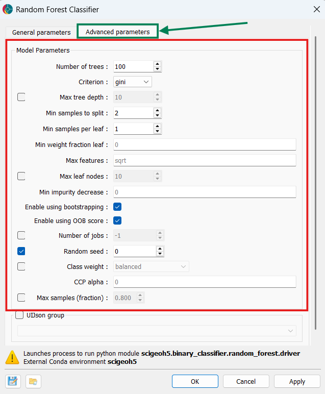
Advanced parameters

The application exposes additional parameters under two collapsible groups: Model Parameters, and Output. All Model Parameters are automatically disabled when a pretrained model is loaded.

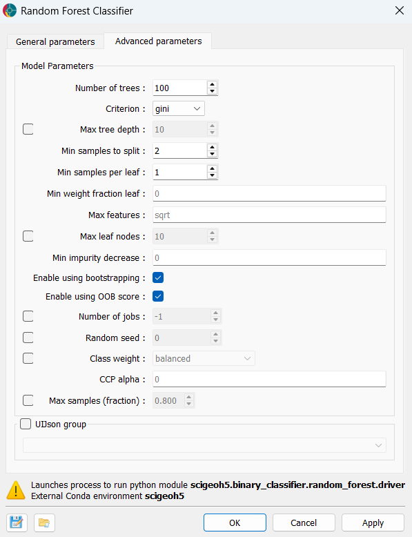
Model Parameters

These settings are only active in training mode. They are all disabled when a **Model file* is selected.

Ensemble structure

• Number of trees (default = 100, min = 1): The number of decision trees in the ensemble. More trees generally improve accuracy and reduce variance at the cost of longer training and prediction times.

• Criterion (default = “gini”): The function used to measure split quality. "gini" measures Gini impurity; "entropy" and "log_loss" both measure information gain. In practice, results are often similar across all three options.

Tree complexity

• Max tree depth (optional, unconstrained by default, min = 1): The maximum depth of each tree. When disabled, trees are grown until all leaves are pure or have fewer than Min samples to split samples. Shallower trees reduce overfitting at the cost of some accuracy.

• Max leaf nodes (optional, unconstrained by default, min = 2): Limits the total number of leaf nodes per tree, growing trees in a best-first fashion. Useful as an alternative way to constrain complexity alongside Max tree depth.

• CCP alpha (default = 0.0, min = 0.0): Complexity parameter for Minimal Cost-Complexity Pruning. Increasing this value prunes more aggressively, producing smaller, simpler trees. A value of 0 disables pruning.

Split and leaf constraints

• Min samples to split (default = 2, min = 2): Minimum number of samples required to split an internal node. Increasing this helps prevent trees from memorising very specific input-target relationships in the training data and can reduce overfitting.

• Min samples per leaf (default = 1, min = 1): Minimum number of samples required at any leaf node. Increasing this smooths the model, particularly in regions sparse in training data.

• Min weight fraction leaf (default = 0.0, range [0.0, 0.5]): Minimum weighted fraction of the total sample weight required at a leaf. Non-zero values are mainly relevant when sample weights vary.

• Min impurity decrease (default = 0.0, min = 0.0): A node is only split if the impurity decrease is at least this value. Increasing it prunes low-value splits.

• Max features (default = “sqrt”): Number of features considered at each split. Accepted values:

  • "sqrt" — square root of the total feature count (recommended for classification).

  • "log2" — base-2 logarithm of the total feature count.

  • An integer >= 1 — exact number of features.

  • A float in (0.0, 1.0] — fraction of features.

Bootstrap and sampling

• Enable using bootstrapping (default = enabled): When enabled, each tree is trained on a bootstrap sample (random draw with replacement). Disabling this uses the full training dataset for every tree. Both OOB score and Max samples require bootstrapping to be enabled.

• Enable using OOB score (default = enabled, requires bootstrapping): Evaluates each training sample against the trees that did not include it in their bootstrap sample, producing an internal generalisation estimate without a separate validation set. The OOB score is logged to the console after training.

• Max samples (fraction) (optional, range (0.0, 1.0], requires bootstrapping): Fraction of training samples drawn for each tree’s bootstrap sample. When disabled, each bootstrap sample is the same size as the full training set. Reducing this value increases diversity between trees at the cost of individual tree accuracy.

Class handling

• Class weight (optional): Adjusts the contribution of each class during training to account for class imbalance:

  • Disabled (default) — all classes have equal weight.

  • "balanced" — weights are inversely proportional to class frequencies in the full training set.

  • "balanced_subsample" — same as "balanced", but recomputed from each tree’s bootstrap sample.

Computation

• Number of jobs (optional): Number of parallel jobs for fitting and predicting. When disabled (default), a single job is used. Set to -1 to use all available processors. Reduces wall-clock time but increases memory usage.

Reproducibility

• Random seed (optional): Integer seed for the random number generator. When set, two runs with identical inputs produce identical results. When disabled, a different random state is used each time.

Methodology

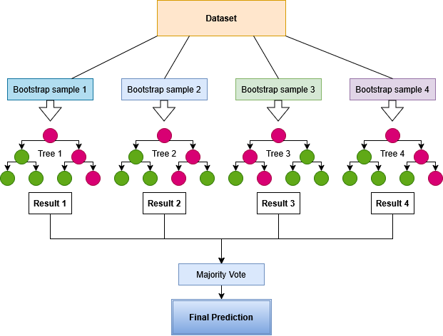
Random Forest builds an ensemble of decision trees. By default (Enable using bootstrapping is on), each tree is trained on a bootstrap sample — a random draw with replacement from the training data — so each tree sees a slightly different subset of examples. When bootstrapping is disabled, every tree is trained on the full training set. At each node split, only a random subset of features is considered (controlled by Max features), which decorrelates the trees and reduces variance.

During prediction, every tree in the ensemble produces a probability estimate for each class by averaging the class fractions in the leaf nodes reached by the input. The application takes the class with the highest mean probability across all trees as the final predicted label (equivalent to a soft-majority vote).

Out-of-Bag (OOB) score: When bootstrapping is enabled, each training sample is excluded from roughly one-third of the trees that were not fitted on it (the “out-of-bag” trees). Passing each sample through its out-of-bag trees produces an internal generalisation estimate. The OOB score is logged after training and ranges from 0 to 1 (higher is better).

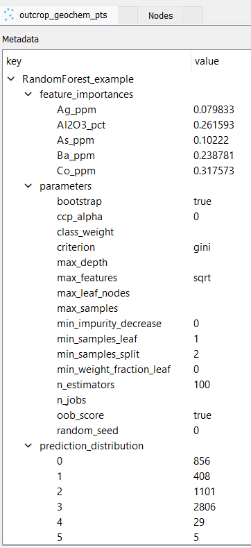
Feature importances: After training, the mean decrease in impurity (Gini importance) is computed for each input feature across all trees. This provides a metric of how much each feature contributed to the model’s predictions. All feature importances are stored in the client object’s metadata.

Output and its limitations

The predicted class label for each data point is the class receiving the highest mean probability across all trees. Per-class probabilities are calibrated estimates of confidence, and they reflect the proportion of trees voting for each class. The model assigns class 0 (Unknown) to any point with missing feature values, which should be interpreted carefully, as an Unknown prediction does not carry any predictive meaning.

Each individual decision tree partitions the feature space using a series of linear threshold rules, i.e. “if feature X > threshold, go left; otherwise, go right”. As a result, a Random Forest can only detect trends based on thresholds; it has no mechanism to capture smoothly curved boundaries or interactions that cannot be expressed as combinations of individual feature thresholds.

More critically, a Random Forest has no built-in concept of spatial relationships. It treats each data point as an independent, identically distributed observation and is entirely blind to proximity, spatial continuity, or geographic structure in the data. Spatial relationships such as grade continuity along a drillhole, or proximity to a fault, cannot be captured by this model.

Data preparation and validation pitfalls

The quality of a Random Forest model is highly sensitive to how the input data are prepared. The following issues should be addressed before training:

• Data leakage: Leakage occurs when information from outside the training set influences the model, causing evaluation metrics to be optimistically biased. Some of the most common sources of this are:

  • Label-encoded inputs: including a feature that directly encodes or is derived from the target label (e.g. a lithology score computed from the same assay used to define the classes). The model learns to predict the label from itself rather than from independent measurements.

  • Spatial leakage from random splitting: in geoscientific datasets, nearby samples are typically more similar than distant ones. A purely random train-test split places spatially close samples on both sides of the split, causing the model to appear more generalisable than it actually is. Where possible, use spatially disjoint splits (e.g. by drillhole or region) to obtain a realistic out-of-sample estimate.

  • Transformation leakage: if normalisation, feature selection, or resampling is computed on the full dataset before splitting, statistics from the test set leak into training. All transformations must be fitted on the training set only and applied separately to the test set.

• Class imbalance: When one class is substantially more frequent than others, the model is biased towards the majority class, and accuracy can appear high even if minority classes are predicted poorly. The most effective remedy is resampling the training data before running this application — typically by undersampling the majority class (randomly removing samples until classes are balanced) or, less commonly, oversampling the minority class. Within this application, the Class weight parameter adjusts the loss function to penalise majority-class errors more heavily, but does not change the underlying sample distribution. Use balanced accuracy, which is logged after training, together with per-class recall stored in the output metadata, to diagnose whether imbalance is affecting results.

• Representativeness of training labels: The model learns only the input-target correlations present in the labelled training samples. If those labels are spatially clustered, biased towards particular lithologies or conditions, or contain labelling errors, the resulting predictions will reflect those biases across the entire prediction domain.

Results

The application writes a single output Referenced property to the client object. Each data point receives the predicted class label (an integer key from the target’s value map), or 0 (Unknown) if that point had missing feature values.

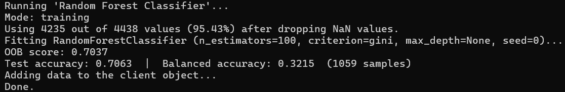
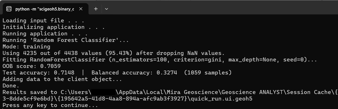
The following information is logged to the application console during a training run:

• Valid sample count: The number of data points with complete feature values, as a fraction of the total, after dropping rows with any no-data value.

• OOB score (training mode only, when bootstrapping is enabled): The out-of-bag generalisation estimate computed from the bootstrap samples not used during each tree’s training.

• Test accuracy and balanced accuracy (training mode only): The fraction of correctly predicted labels on the held-out Test rows, alongside the balanced accuracy (mean per-class recall), and the number of test samples evaluated.

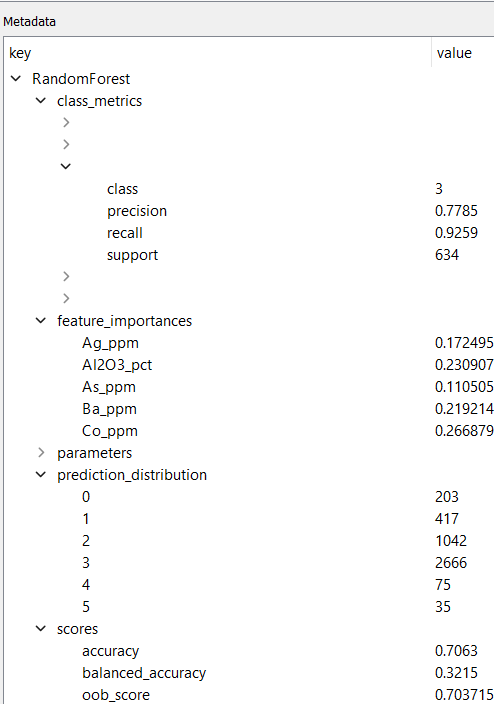
The following information is stored in the client object’s metadata under the output property name and is accessible after the run:

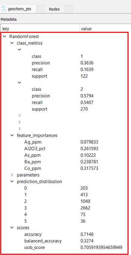
• Parameters: The full set of hyperparameters used for the run, for reproducibility.

• Feature importances: Mean decrease-in-impurity importance for every input feature, sorted in descending order.

• Prediction distribution: The count of data points assigned to each predicted class.

• Scores (training mode only): Test accuracy, balanced accuracy, and OOB score (when enabled).

• Per-class metrics (training mode only): Precision (the fraction of all predictions of a class that are correct), recall (the fraction of members of a class that were correctly identified), and support (the number of samples in the test set belonging to each class).

Tutorial

The following steps describe how to run the Random Forest Classifier application from start to finish, with example screenshots from the interface. The tutorial assumes the user has already prepared an object with appropriate input data and target properties, as well as a train-test split property if running in training mode.

Training Mode

1. Open the Random Forest Classifier application.

2. Select your desired input object, feature properties (data), target property, and train-test split property, as described in the Input section above, by either dragging and dropping from the Objects panel or using the dropdown selectors.

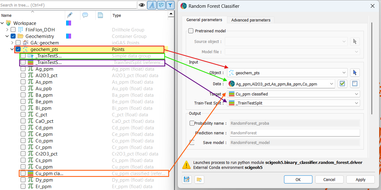
3. In the Output section, specify a name for the output prediction property if desired, and optionally enable Probability name to produce per-class probability output properties. You can also enable Save model to attach the trained model as a .pkl file to the client object for later reuse in inference mode.

4. Optionally, adjust any model parameters in the Advanced Parameters > Model Parameters section to control the ensemble structure, tree complexity, split constraints, and other aspects of the training process. For example, it is recommended to fix a random seed for reproducibility.

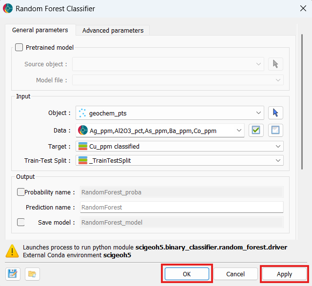
5. Click the OK button to close the Random Forest Classifier UI and run the application, or Apply to run without closing the UI. The console will log the training progress and results, and the output properties will be written to the client object once complete.

6. Examine the results: the predicted classes in the output property, the prediction probabilities (if enabled), and the metadata containing feature importances, diagnostics, and other metrics.

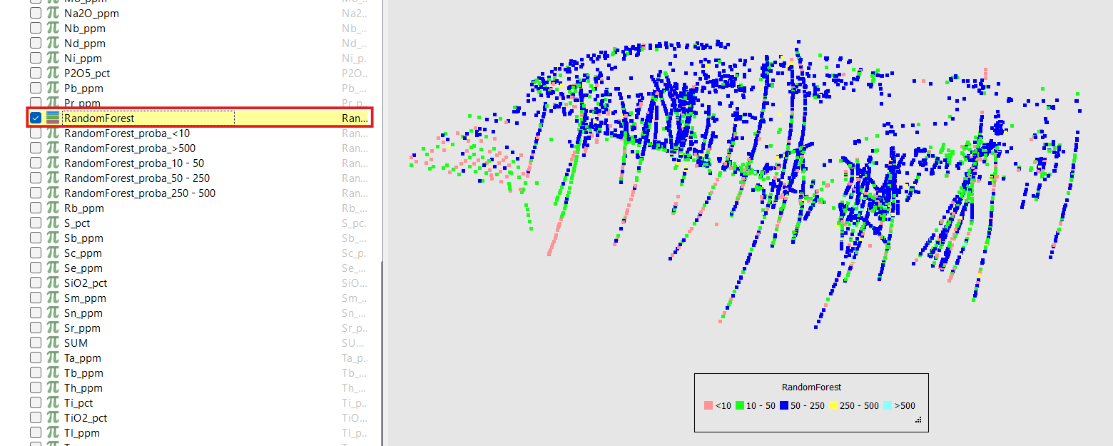
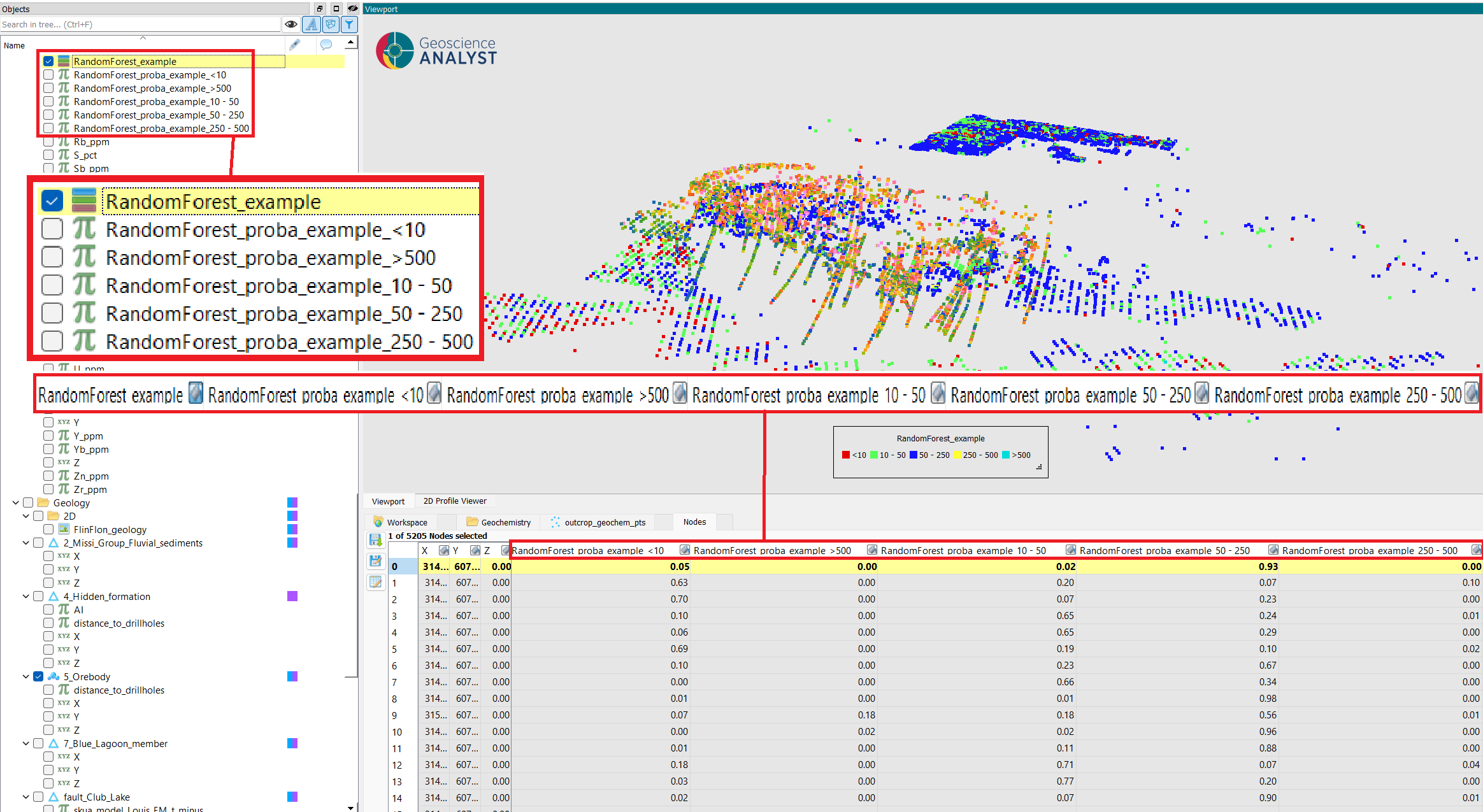
Predicted classes in the output property:

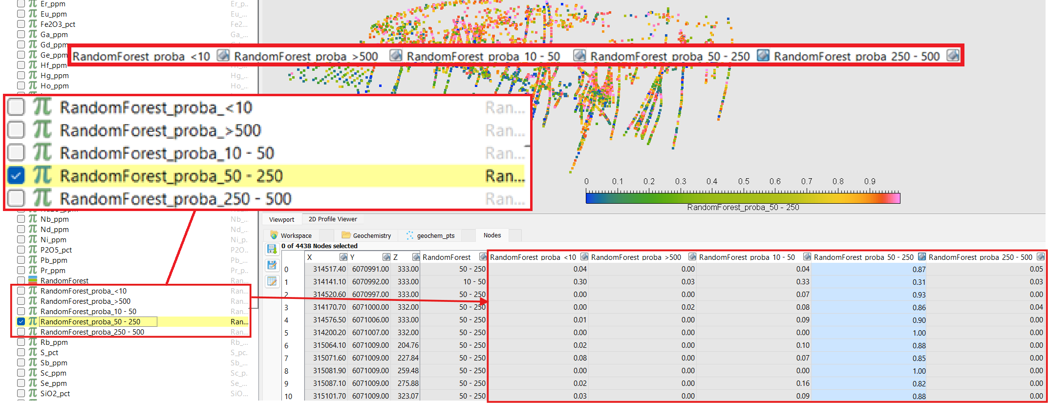
Predicted probabilities (if Probability name was enabled):

Feature importances and metrics in the output metadata:

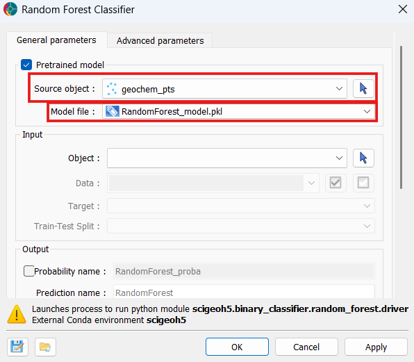
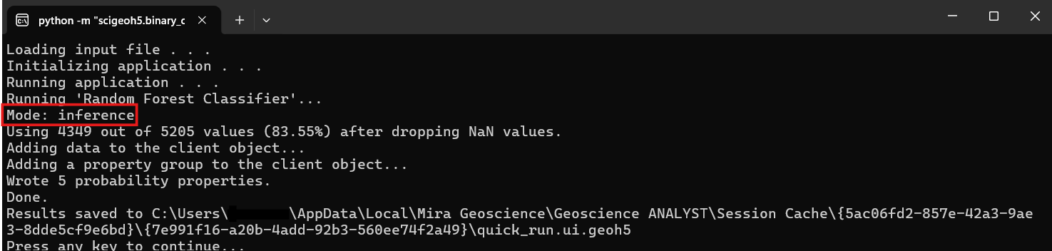
Inference Mode

The inference mode tutorial assumes a model has already been trained and saved via Save model in a previous training run (see step 3 above).

1. Open the Random Forest Classifier application and enable the Pretrained model group by checking the group checkbox.

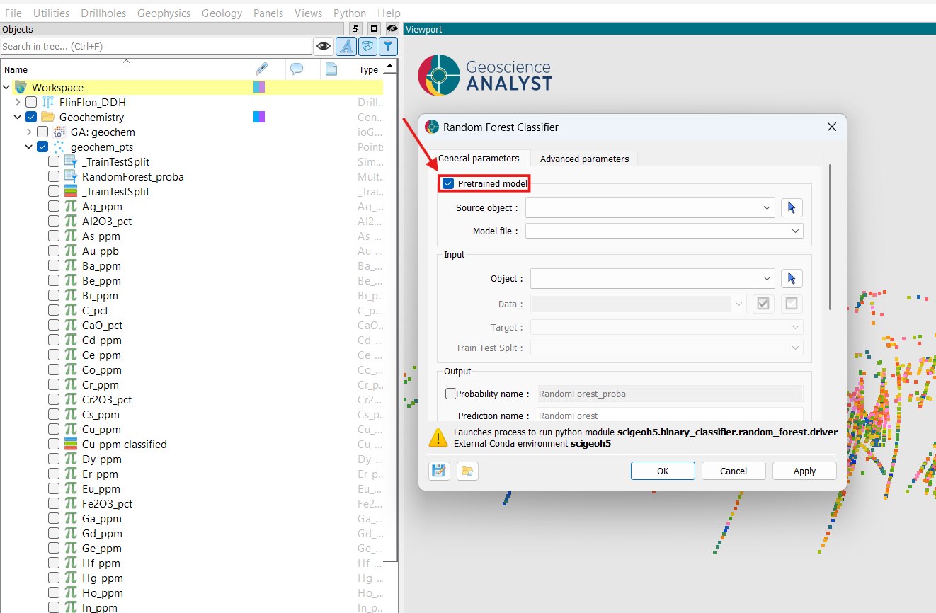
2. Select the Source object — the object to which the .pkl file was saved during training. Then select the .pkl file from the Model file dropdown.

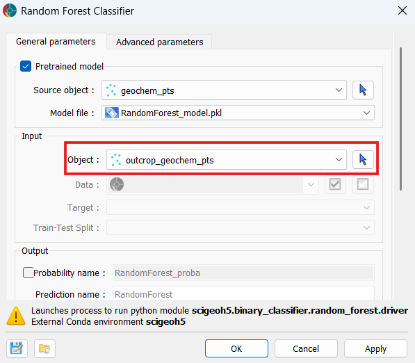
3. Select the Object to predict on. This can be the same object used during training or a different one, provided it contains properties with the same names as the features the model was trained on. All other input fields are disabled automatically.

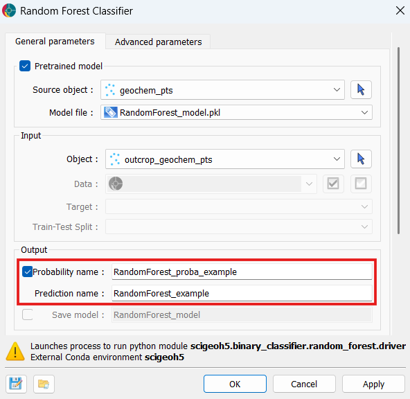
4. Optionally, specify a Prediction name and enable Probability name in the Output section.

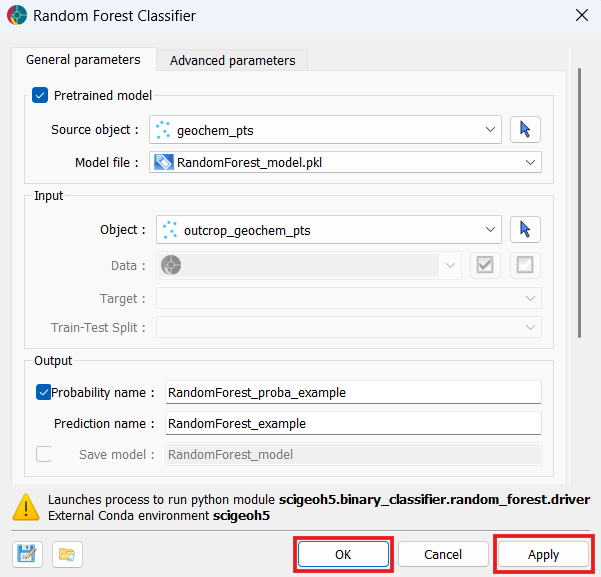
5. Click OK or Apply to run. No training occurs — predictions are produced directly from the loaded model and written to the selected object.

6. Examine the results: the predicted classes and probability properties (if enabled) written to the object, and the metadata containing feature importances and prediction distribution.

Output properties written to the object:

Output metadata: